Practical Graph Isomorphism
the individualization-refinement method
				
				
					Isomorphism and Automorphism
				
                
				  We have some finite objects consisting of some finite sets 
                    and some relations on them. 
                    An isomorphism between two objects is a bijection 
                    between their sets so that the relations are preserved. 
                    Isomorphism is an equivalence relation on the set of all objects.
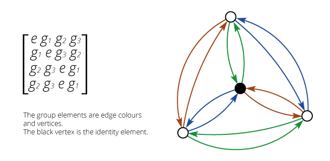
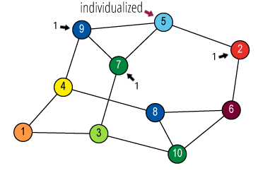
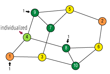
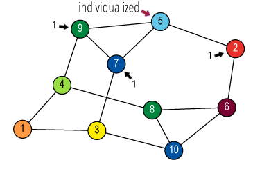
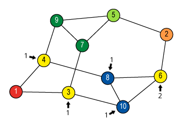
					Isomorphisms from an object to itself are automorphisms. 
                    The set of automorphisms forms a group under composition.
					It is called the automorphism group.
                     (1)
                    
                    (1)
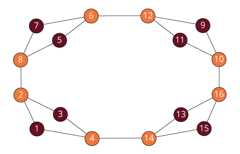
					(1 4) (2 3) (5 8) (6 7)
					(1 8) (2 7) (3 6) (4 5)
					(1 5) (2 6) (3 7) (4 8) 
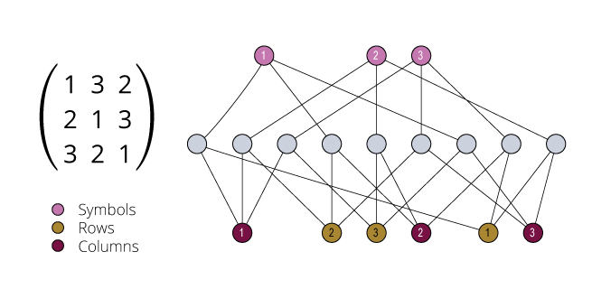
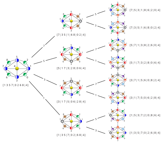
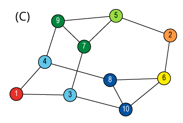
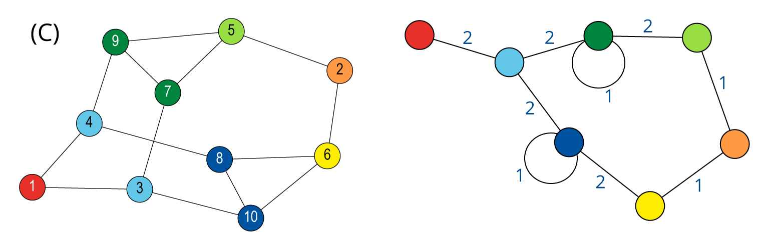


					The graph isomorphism problem is: (GI) 
                    Given two graphs, determine whether they are isomorphic.
					The fastest known algorithm for GI is 
                    quasipolynomial; 
                    no polynomial time algorithm is known (despite many claims).
					GI is not known to be NP-complete. GI is not known to be in co-NP.
					There are polynomial time algorithms for many special classes of graphs 
					(bounded degree, bounded genus, classes with excluded minors or topological 			
                    subgraphs). Few of these are practical, planar graphs being a notable exception.
					It is possible that group isomorphism is easier and that permutation
                    equivalence of linear codes is harder than GI. But nobody can prove it.


Ubiquity of Graph Isomorphism
Very many isomorphism problems can be efficiently expressed as graph isomorphism
problems. For convenience, we use coloured graphs, in which the vertices (and possibly
the edges) are coloured. Isomorphisms must preserve vertex and edge colour.


Matrix Isomorphism


Hadamard Equivalence


Isotopy


Group Isomorphism


				Given a class of objects, and a definition of isomorphism, 
                we can choose one member of each isomorphism class and call it the 
                canonical member of the class.
				The process of finding the canonical member of the isomorphism class containing 
                a given object is called canonical labeling.
				Two labeled objects which are isomorphic become identical when they are 
                canonically labeled. 
                Since identity of objects is usually far easier to check than isomorphism,
				canonical labeling is the preferred method of sorting a collection of objects 
                into isomorphism classes.
				A possible definition of the canonical member of an isomorphism class would be 
                the member which maximises some linear representation (such as a list of edges).
				In practice, most programs compute a canonical member which is easy for 
                computers to find rather than easy for humans to define.


					Refinement: equitable partition
				
                
				A key concept used by nauty and other tools is 
                partition refinement  (partition = colouring).
				An equitable partition is one where every two vertices of the same colour are 		
                adjacent to the same number of vertices of each colour.
                
                 
                Equitable partitions


					Refinement of a partition means to subdivide its cells.
					Given a partition (colouring) π, there is a unique equitable partition 
                    that is a refinement of π and has the least number of colours.
                    The next picture shows the steps which lead from an initial colouring to 
                    the equitable partition. The black arrows indicate vertices having a
                    number of neighbours in a reference cell which is different from that of other
                    vertices in their cell.


                Refinement steps


					All competitive isomorphism programs generate a tree based on 
                    partition refinement. The nodes of the tree correspond to partitions (colourings).
					The root of the tree corresponds to the initial colouring, refined.
					If a node corresponds to a discrete partition 
                    (each vertex with a different colour), it has no children and is a leaf.
					Otherwise we choose a colour used more than once (the target cell), 
                    individualize one of those vertices by giving it a new unique colour, and refine 
                    to get a child.
					Each leaf lists the vertices in some order (since colours have a predefined order),
                    so it corresponds to a labelling of the graph.
					If we have two leaves giving the same labelled graph, 
                    we have found an automorphism.
					If we define an order on labelled graphs, such as lexicographic order, 
                    then the greatest labelled graph corresponding to a leaf is a canonical graph.
					However the tree can be much too large to generate completely.
                    It will be pruned by means of node invariants.


					Node invariants and pruning
				
                
				A 
node invariant is a value Φ(ν) attached to each node ν 
                in the tree that depends only on the combinatorial properties of ν 
                and its ancestors in the search tree (not on the labelling of the graph).
				Node invariants, together with automorphisms, allow us to remove parts of the search
				tree without generating them.
                
                
				-  If ν1, 
                ν2
                are nodes at the same level in the search tree and
 Φ(ν1) <
                 Φ(ν2), then
					no canonical labelling is descended from ν1.
-  If ν1, 
                ν2
                are nodes at the same level in the search tree and
 Φ(ν1) ≠
                 Φ(ν2), then
					no labelled graph descended from ν1 is the same as one descended from 
                    ν2.
-  If ν1, 
                ν2 
                are nodes with ν2 = 
                (ν1)g
				for an automorphism g, then g maps the subtree
				descended from ν1 
                onto the subtree descended from ν2.
				Each of these observations enables us to prune parts of the search tree.
				The hope is that the remaining parts will be small enough to compute.


                Search tree without pruning
                
    
Equitable Partition and Orbit Partition - An Example
Equitable partitions are in general unable to capture the orbit partition of vertices of
a graph, as shown by the next example: vertices 3, 4, 5 and 6 are in the same cell of the equitable partition but there isn't any automorphism between vertices in {3, 4} and in {5, 6}.


Initial graph


Count neighbours of green vertices


Equitable partition


Orbit partition


    The individualization-refinement method allows − in two steps − 
    for detecting an automorphism which maps vertex 3 into 4. 
    Remark: Assume that an ordered sequence of n 
    (the number of vertices of the graph) colours is given.
    The individualized vertex keeps the colour of the cell to which
    it belongs, while the remaining vertices in that cell are assigned the next colour.


Individualize vertex 3 (green) and count its neighbours


Count neighbours of blue vertices


Equitable partition


Individualize vertex 5 (cyan) and count its neighbours


Equitable (and discrete) partition


Individualize vertex 4 (green) and count its neighbours


Count neighbours of blue vertices


Equitable partition


Individualize vertex 5 (cyan) and count its neighbours


Equitable (and discrete) partition


The automorphism (3 4) (7 9) (8 10)
is found by comparing vertices of the coloured graphs (D) and (D').


					Base and strong generating set - Group size
				
Example of a base and strong generating set. For a graph with n vertices there are at most n − 1 generators, even though the group size can be up to n!


1) Fixing 1,5,9,13


2) Fixing 1,5,9. Orbit of 13 is {13, 15}


3) Fixing 1,5. Orbit of 9 is {9, 11}


4) Fixing 1. Orbit of 5 is {5, 7, 13, 15}


5) Fixing nothing.
Orbit of 1 is {1, 3, 5, 7, 9, 11, 13, 15}


1) Everything fixed.
2) Orbit of 13 is {13, 15} (orbit size=2)
Generator: (13 15)
3) Orbit of 9 is {9, 11} (2)
(9 11)
4) Orbit of 5 is {5, 7, 13, 15} (4)
(5 7),
(2 4)(5 13)(6 16)(7 15)(8 14)(10 12)
5) Orbit of 1 is {1, 3, 5, 7, 9, 11, 13, 15} (8)
(1 3),
(1 5)(2 8)(3 7)(4 6)(9 13)(10 16)(11 15)(12 14)
Group size = 2 × 2 × 4 × 8 = 128.