Search space traversal
in nauty and traces-
-
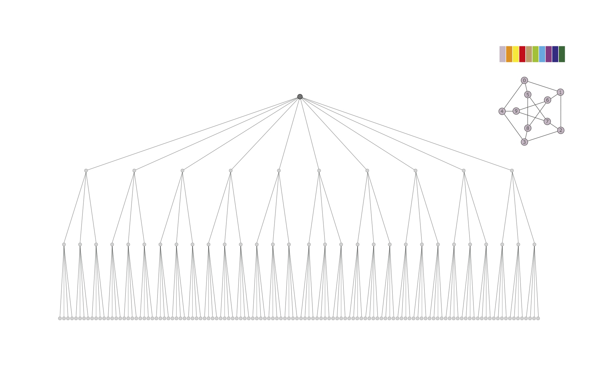
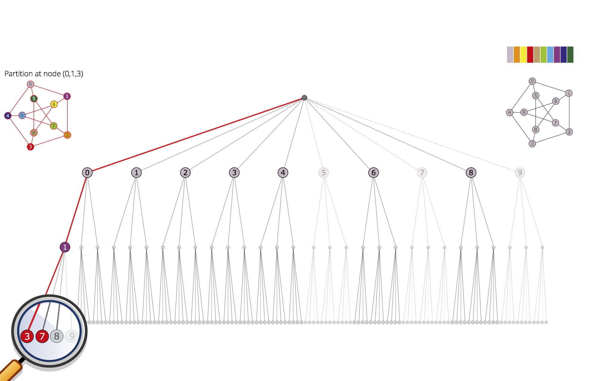
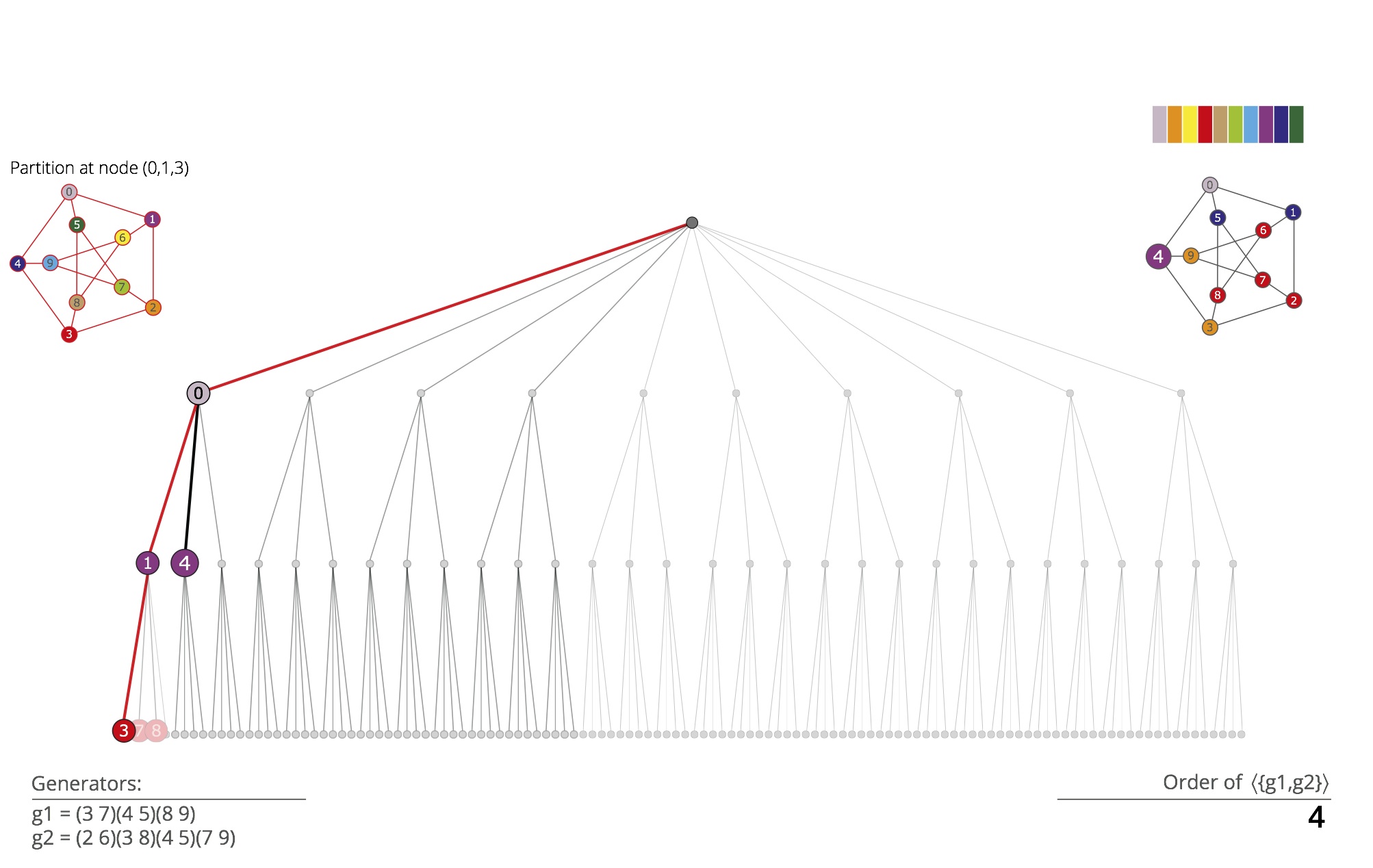
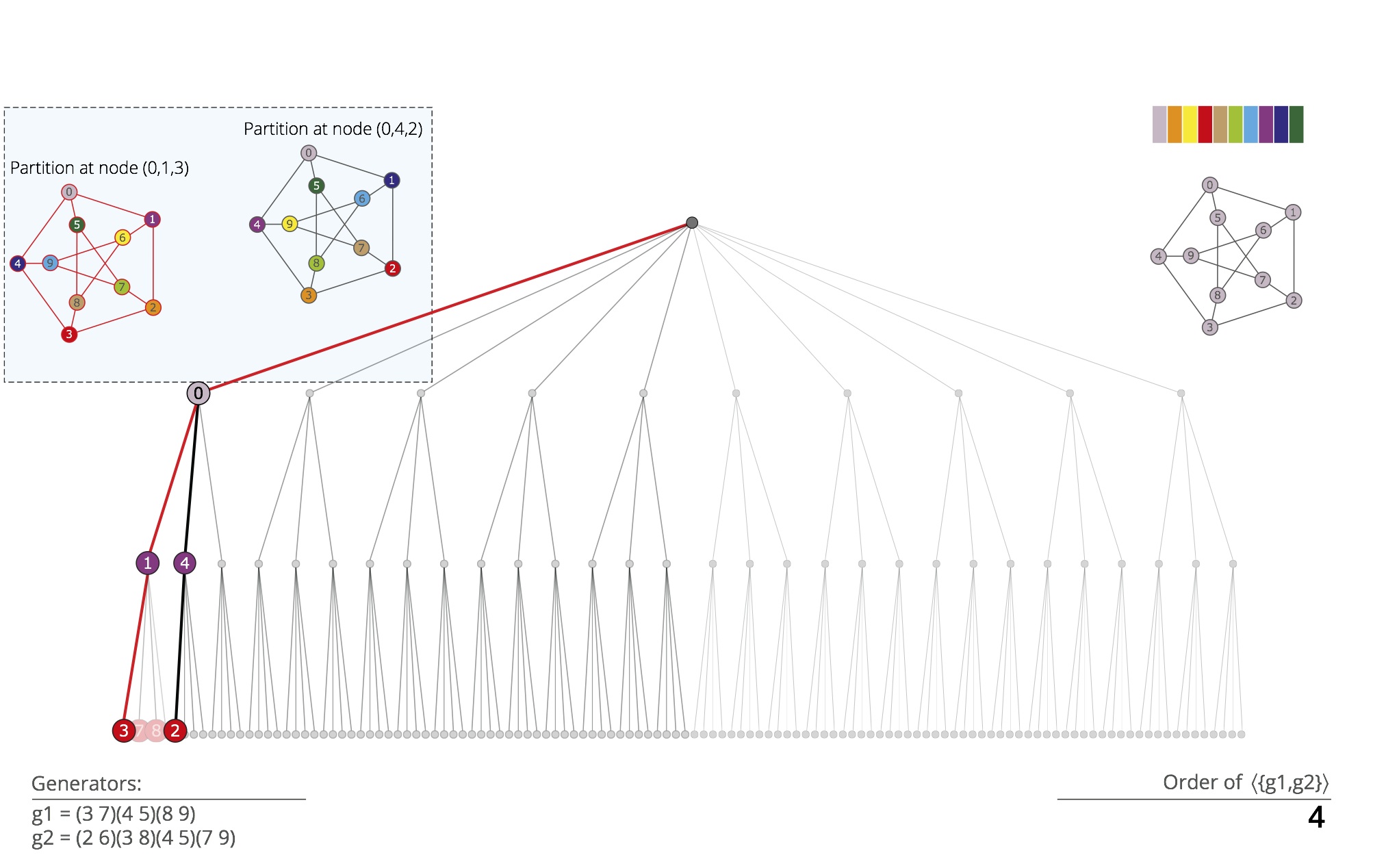
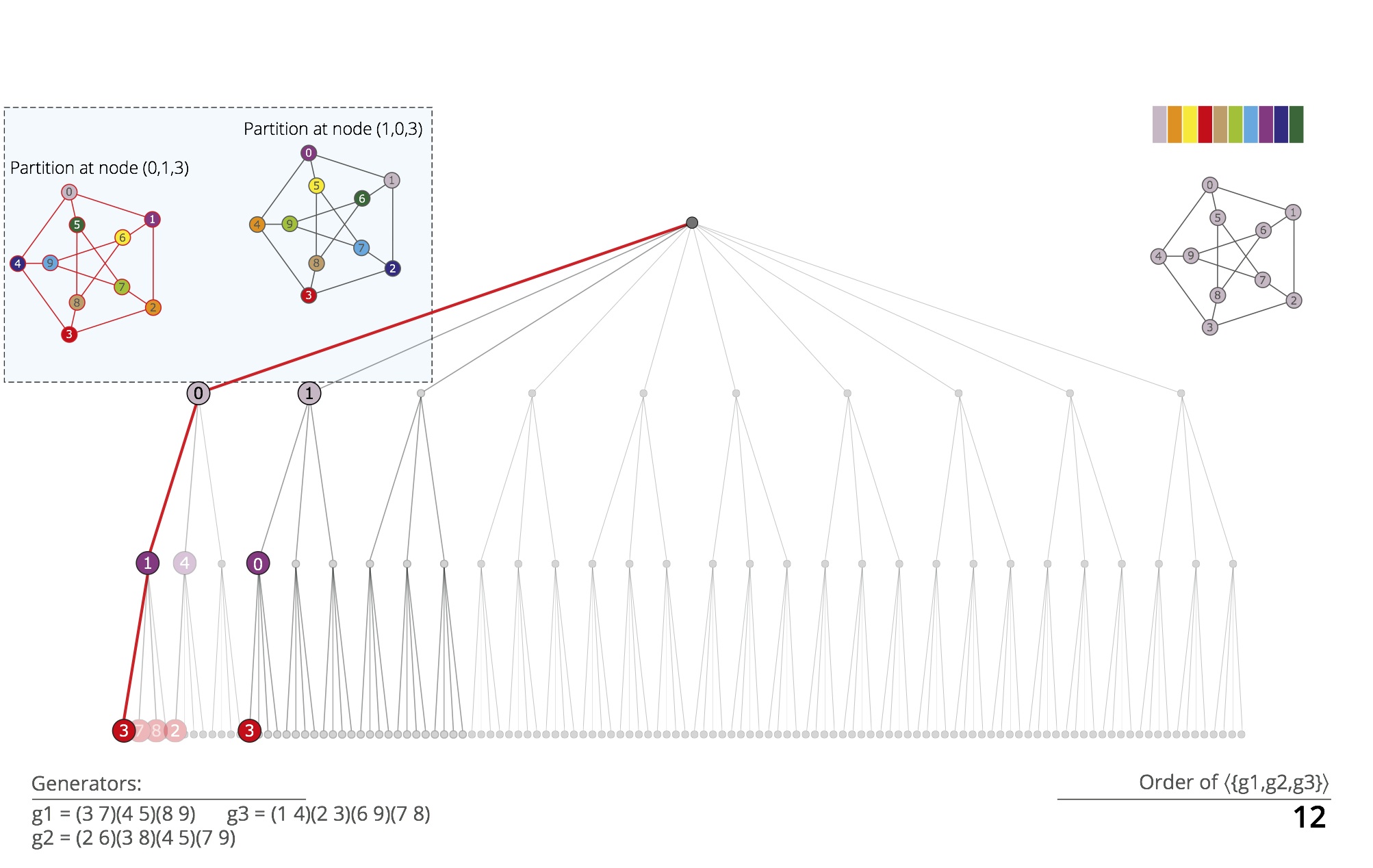
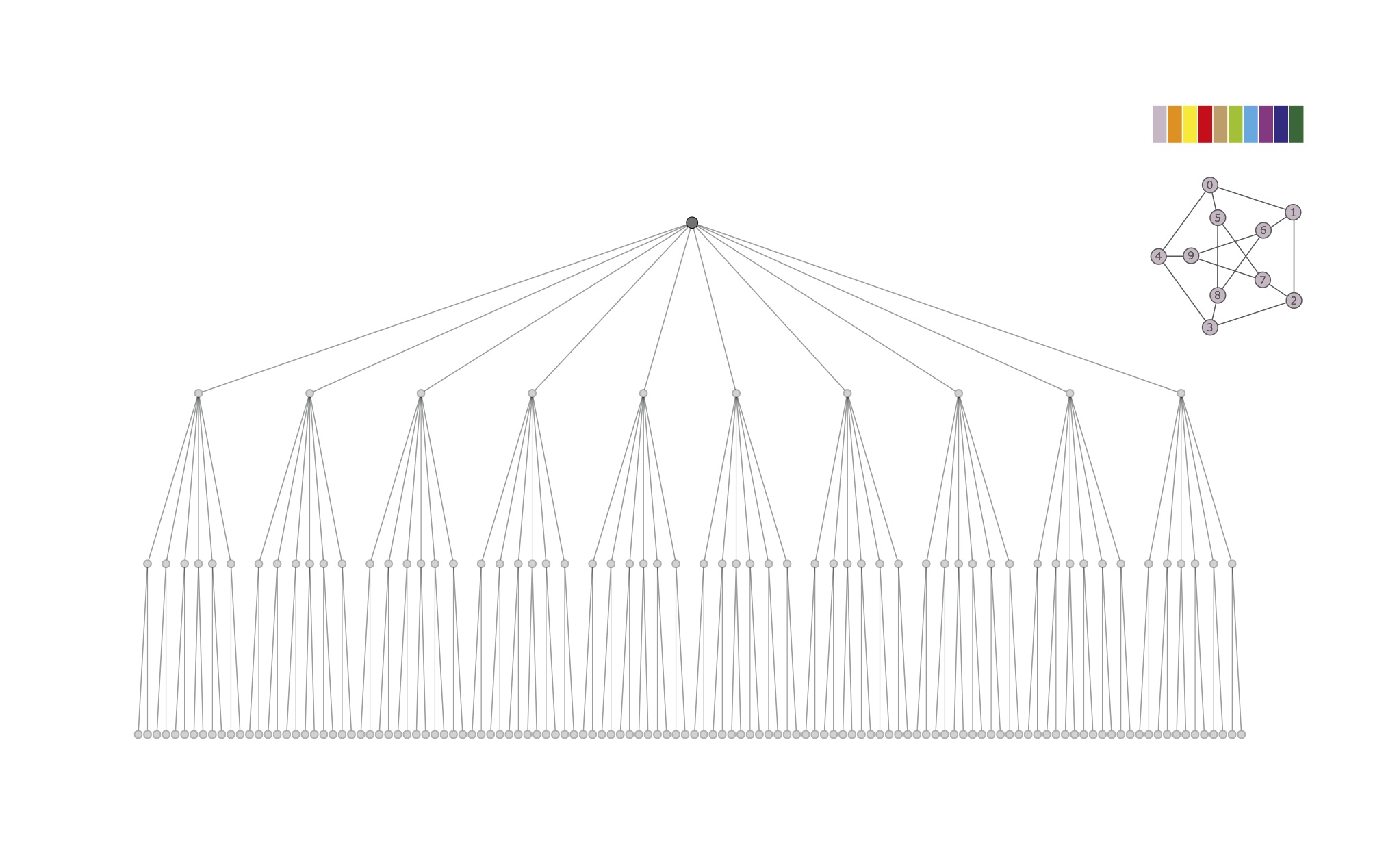
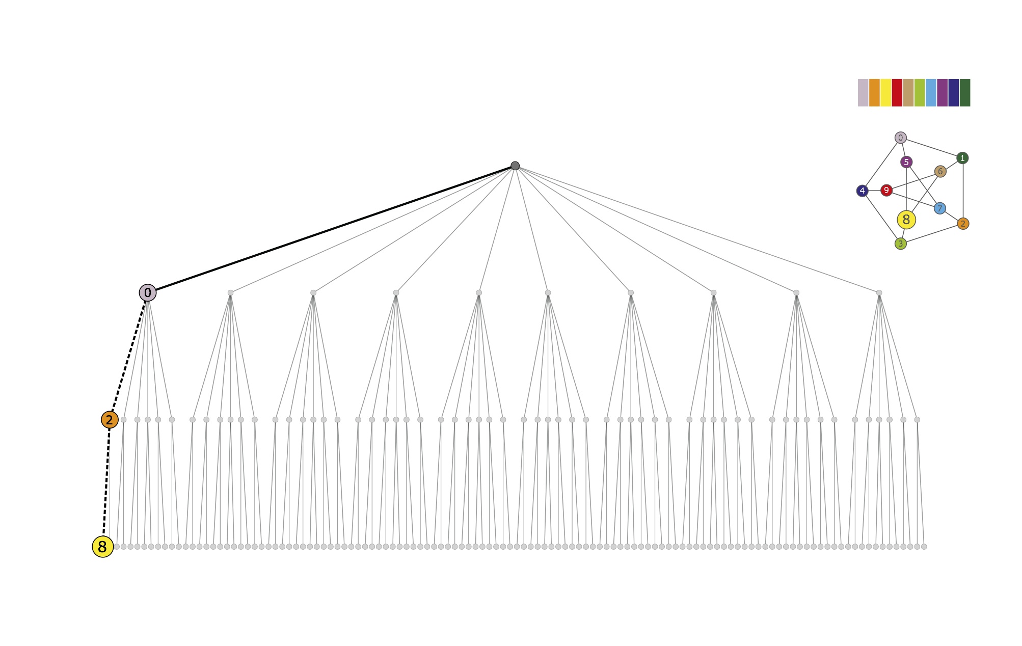
Nauty's search tree. The target cell has size 10 at the topmost level, size 3 at level 2, 4 at level 3, where the individualizations produce discrete partitions. nauty executes a classical backtrack traversal of the tree, pruning it as soon as automorphisms are found.
-

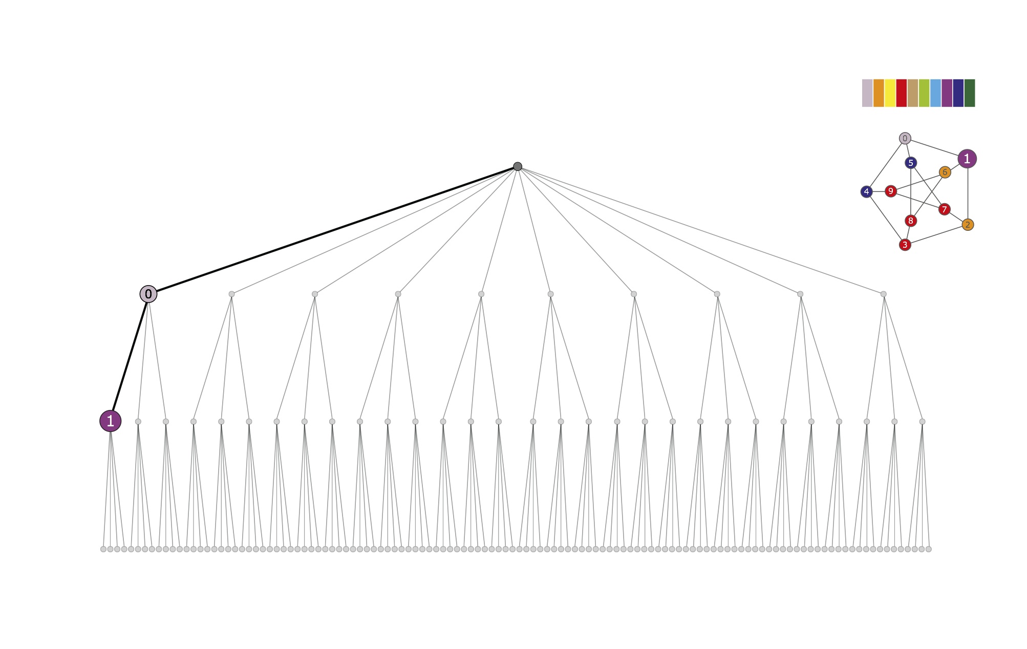
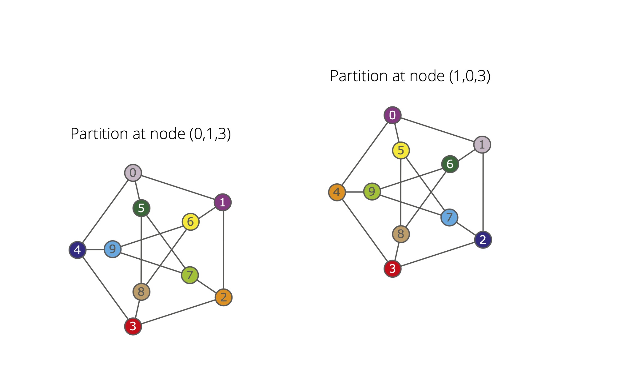
First individualization and refinement. The first vertex in the target cell {0,...,9} is individualized; the corresponding partition [ 0 | 1:9 ] is refined to the equitable partition [ 0 | 2 3 6:9 | 1 4 5 ]. The target cell for the next level is {1,4,5}.
-
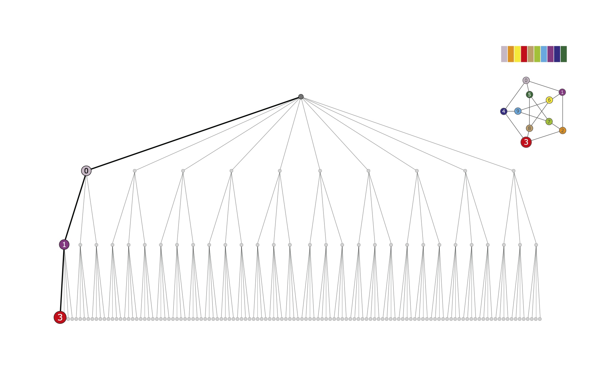
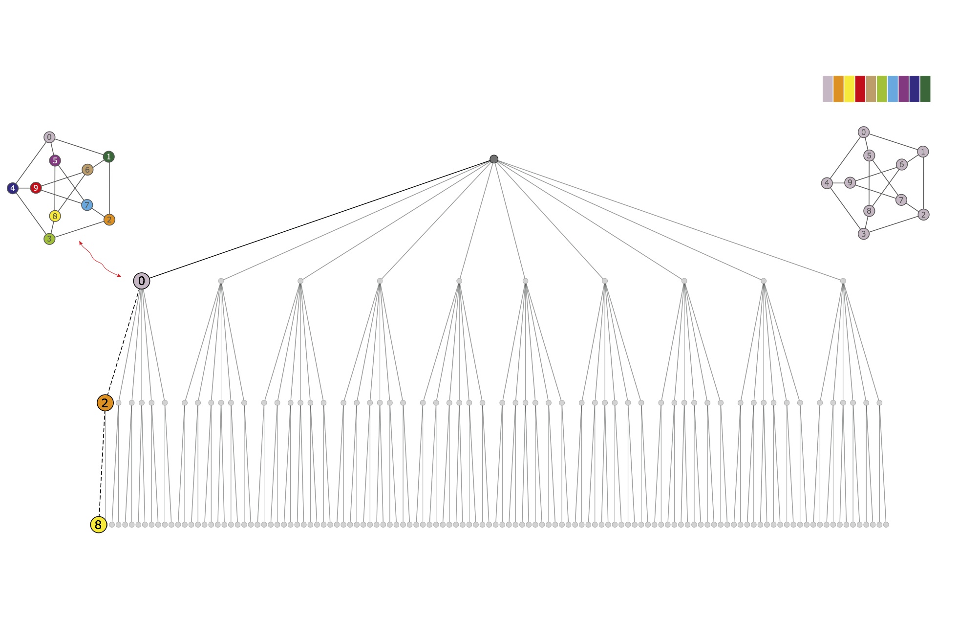
Individualization and refinement. The first vertex in the target cell {1,4,5} is individualized; the corresponding partition [ 0 | 2 3 6:9 | 1 | 4 5 ] is refined to [ 0 | 2 6 | 3 7:9 | 1 | 4 5 ]. The target cell for the next level is {3,7,8,9}.
-
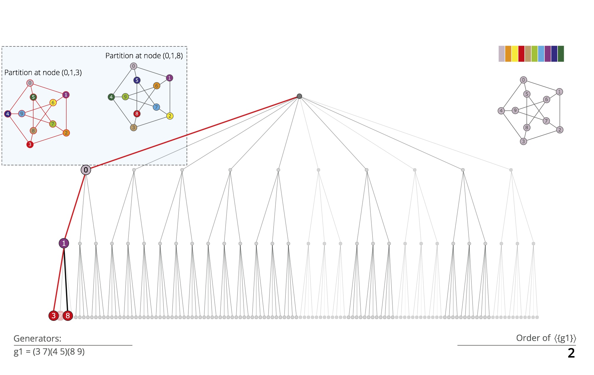
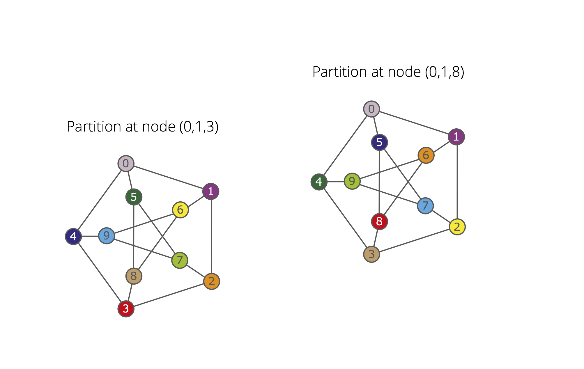
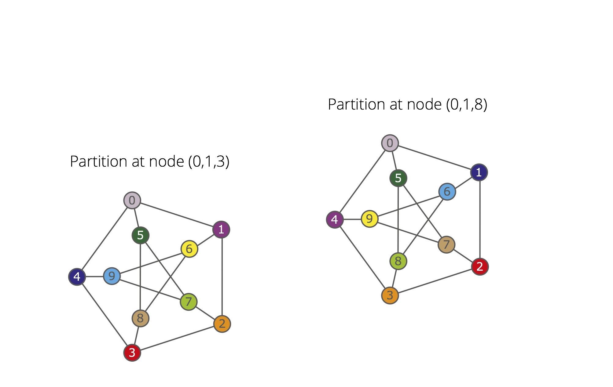
Discrete partition. The first vertex in the target cell {3,7,8,9} is individualized; we obtain the partition [ 0 | 2 6 | 3 | 7:9 | 1 | 4 5 ], which refines to [ 0 | 2 | 6 | 3 | 8 | 7 | 9 | 1 | 4 | 5 ], a discrete partition.
-
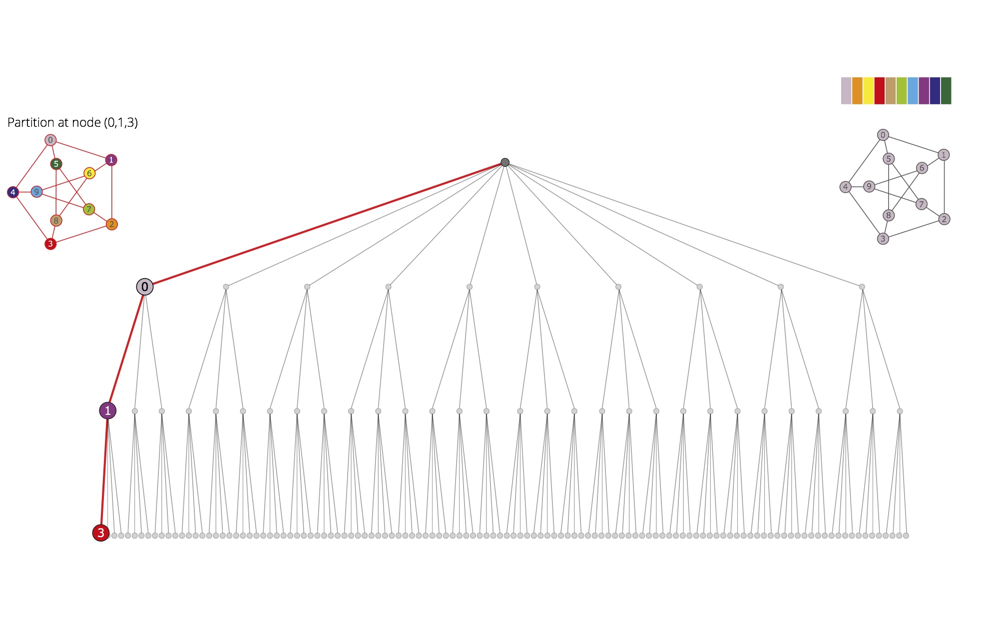
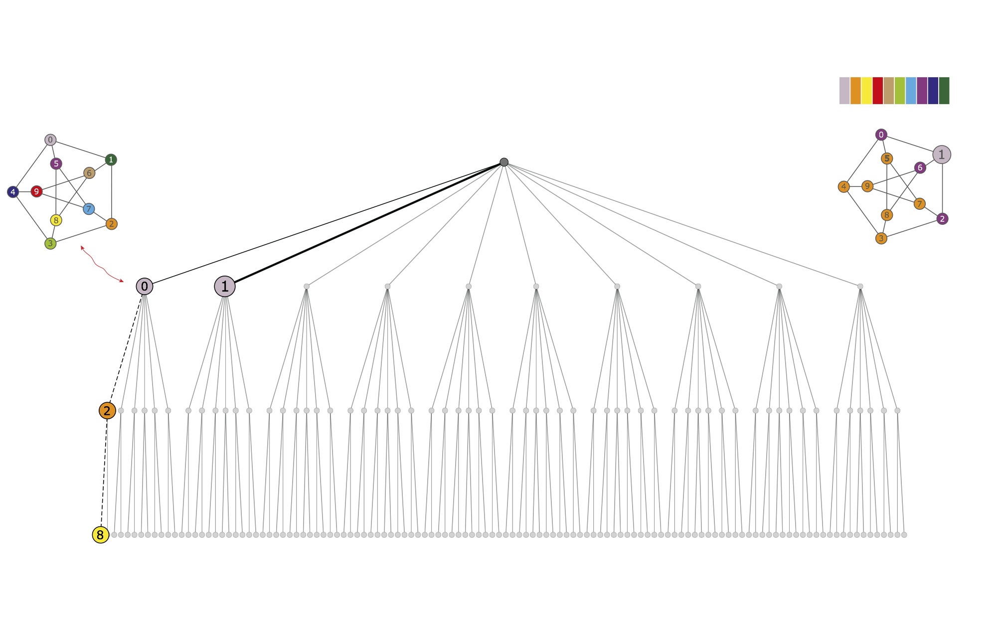
First path and backtrack. The partition obtained at the leaf corresponding to the first individualization-refinement path (0,1,3) is stored for comparison with next partitions. The backtrack search proceeds from the previous level, where the target cell is {3,7,8,9}.
-
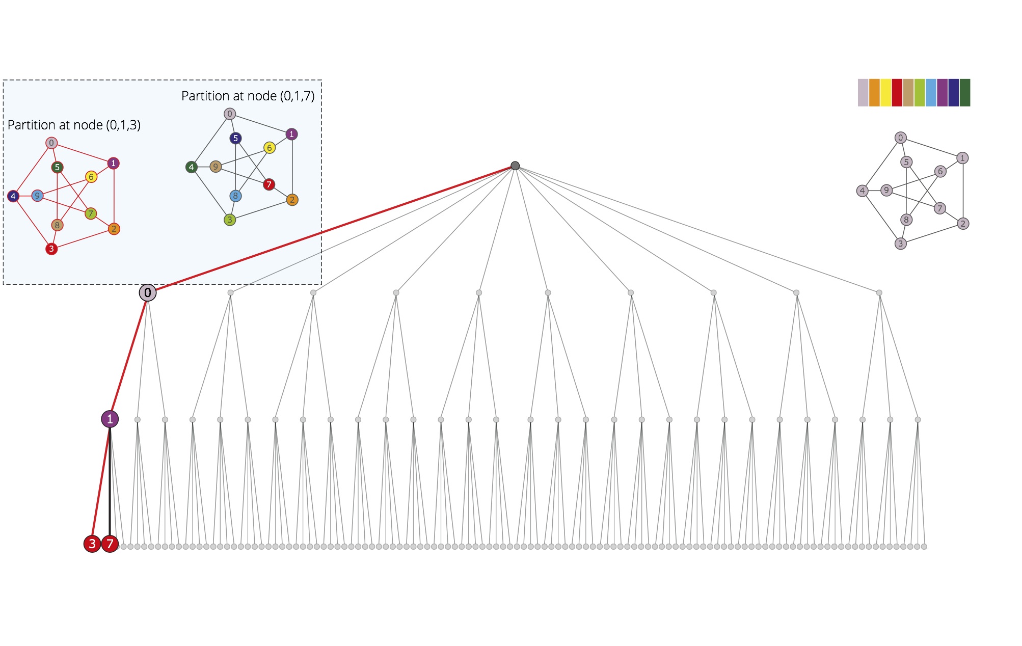
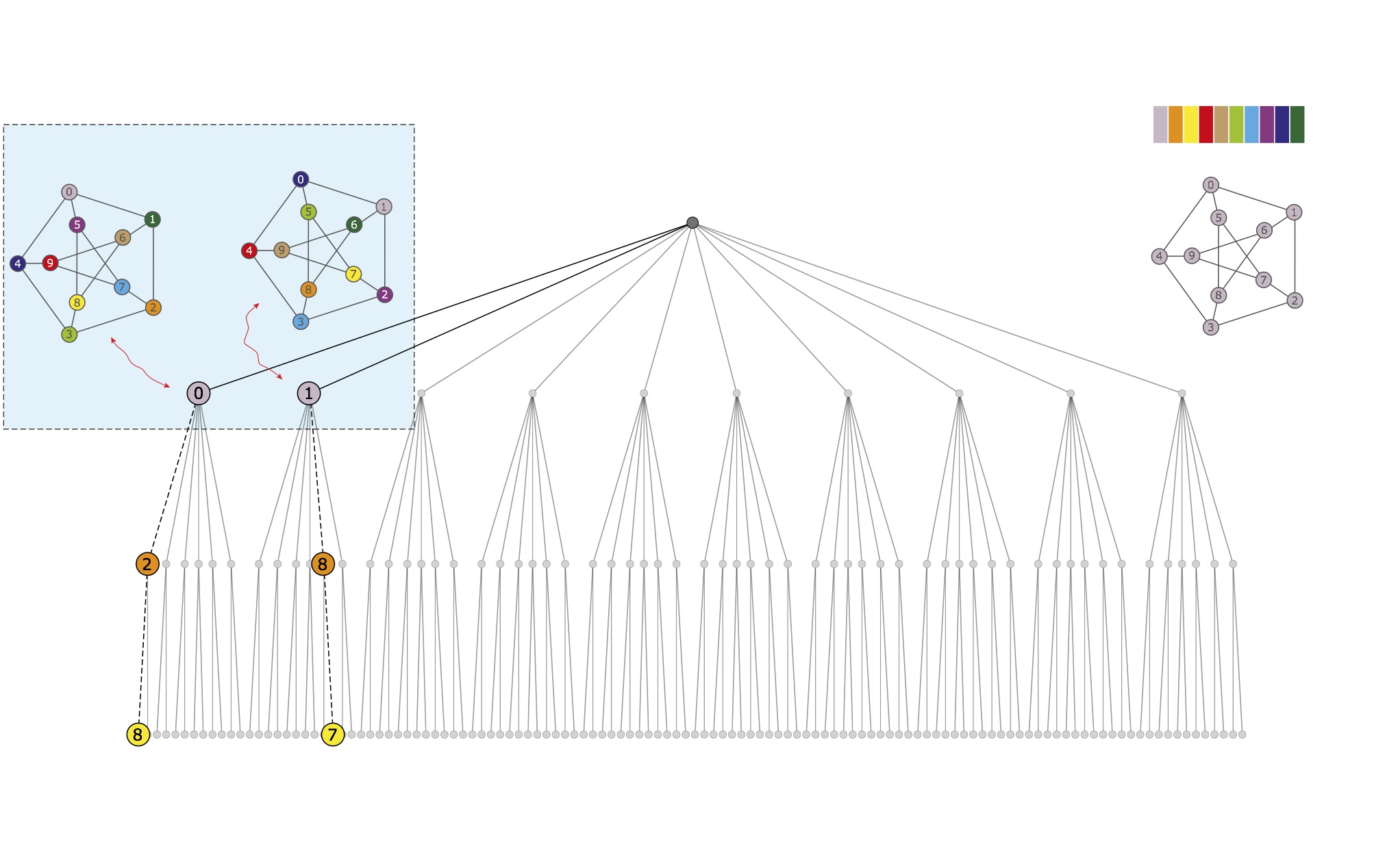
Second discrete partition. The second vertex in the target cell {3,7,8,9} is individualized; we have the partition [ 0 | 2 6 | 7 | 3 8 9 | 1 | 4 5 ], which refines to [ 0 | 2 | 6 | 7 | 9 | 3 | 8 | 1 | 5 | 4 ], a discrete partition.
-
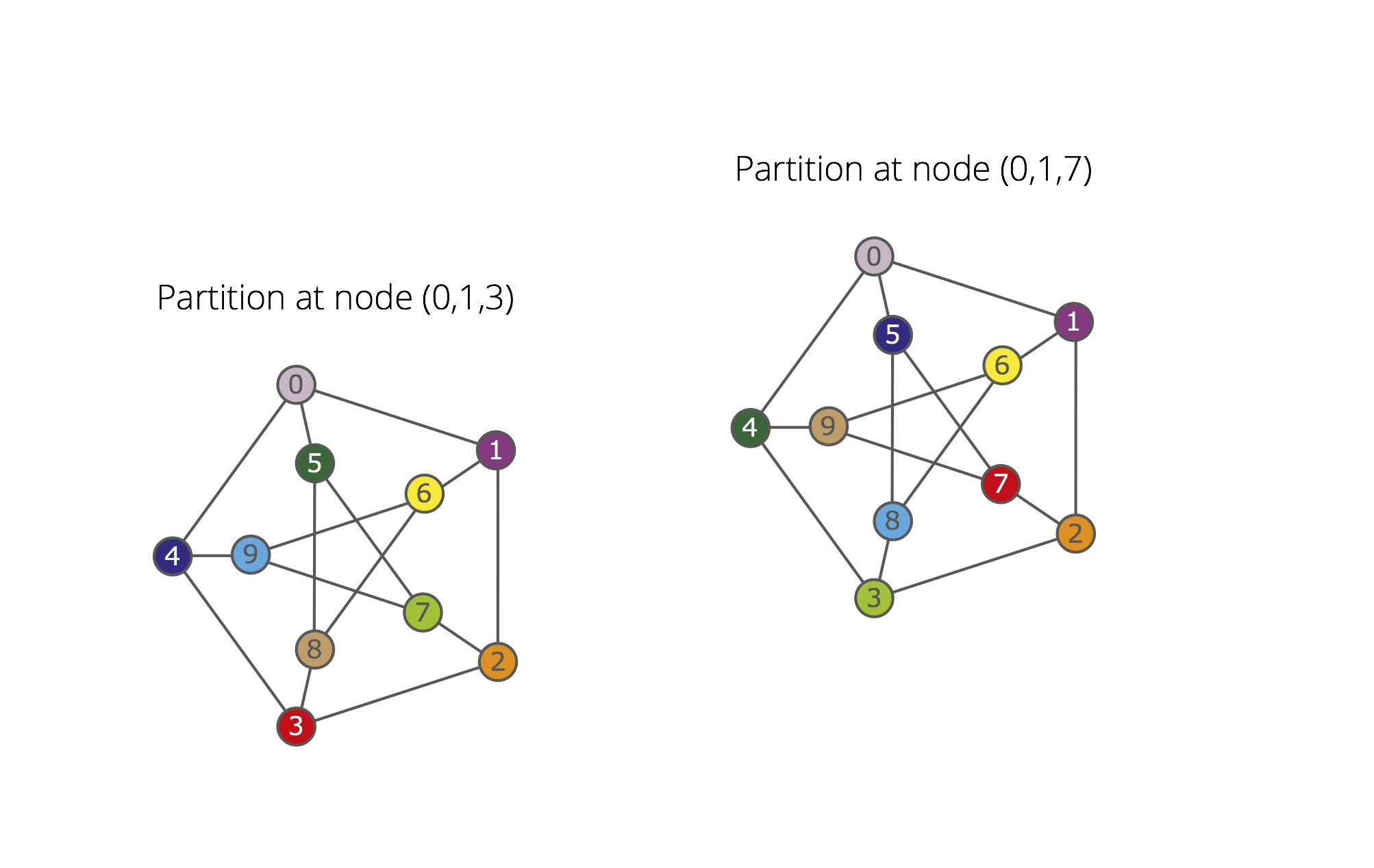
Automorphism. For each color c, the vertices colored by c in the first and in the second graph have neighbors with the same colors. This determines an automorphism, mapping each vertex of the second colored graph to the vertex of the first graph having its color. In this case, (3 7)(4 5)(8 9).
-
Pruning. The detected automorphism g1 = (3 7)(4 5)(8 9) allows for pruning the subtrees rooted at 5, 7, 9 and (0,1,9), since they are equivalent to those rooted at 4, 3, 8 and (0,1,8), respectively. The subgroup generated by g1 has order 2.
-
Backtrack. We go back again to the node (0,1), where we are left with the individualization of the third vertex in the target cell {3,7,8,9}; we obtain the partition
[ 0 | 2 6 | 8 | 3 7 9 | 1 | 4 5 ], which refines to [ 0 | 6 | 2 | 8 | 3 | 9 | 7 | 1 | 5 | 4 ]. -
Automorphism. The comparison between the partitions at (0,1,3) and (0,1,8) determines the automorphism g2 = (2 6)(3 8)(4 5)(7 9). The group ‹{g1,g2}› generated by g1 and g2 has order 4 and orbits {0},{1},{2,6}{3,7,8,9},{4,5}. Therefore, the subtrees rooted at 6 and 8 are pruned.
-
Backtrack. We turn back to node 0 and we individualize the second vertex in the target cell {1,4,5}. After refinement, we obtain the partition [ 0 | 3 9 | 2 6:8 | 4 | 1 5 ]. The target cell for the next level is {2,6,7,8}.
-
Discrete partition. The first vertex in the target cell {2,6,7,8} is individualized; we obtain the partition [ 0 | 3 9 | 2 | 6:8 | 4 | 1 5 ], which refines to [ 0 | 3 | 9 | 2 | 7 | 8 | 6 | 4 | 1 | 5 ], a discrete partition.
-
Automorphism. A new automorphism is found, g3 = (1 4)(2 3)(6 9)(7 8). The group ‹{g1,g2,g3}› has order 12 and orbits {0},{1,4,5},{2,3,6,7,8,9}. The subtrees rooted at 3, 4 and (0,4) are pruned. The subtree rooted at (0,5) is also pruned. In fact, g1, g2 and g3 fix 0, hence {1,4,5} is an orbit of the 0-stabilizer of the generated group: the subtree rooted at (0,5) is equivalent to the one rooted at (0,1).
-
Backtrack. The backtrack search turns back to the root of the tree, and then subsequently individualizes vertices 1, 0 and 3, refining the corresponding partitions. These steps, not detailed here, lead to the discrete partition [ 1 | 4 | 5 | 3 | 8 | 9 | 7 | 0 | 2 | 6 ].
-
Automorphism. A new automorphism is found, g4 = (0 1)(2 4)(5 6)(7 9). The group ‹{g1,g2,g3,g4}› has order 120 and one orbit. The subtrees rooted at 1 and 2 are pruned. The computation of the automorphism group of the input graph stops.
-
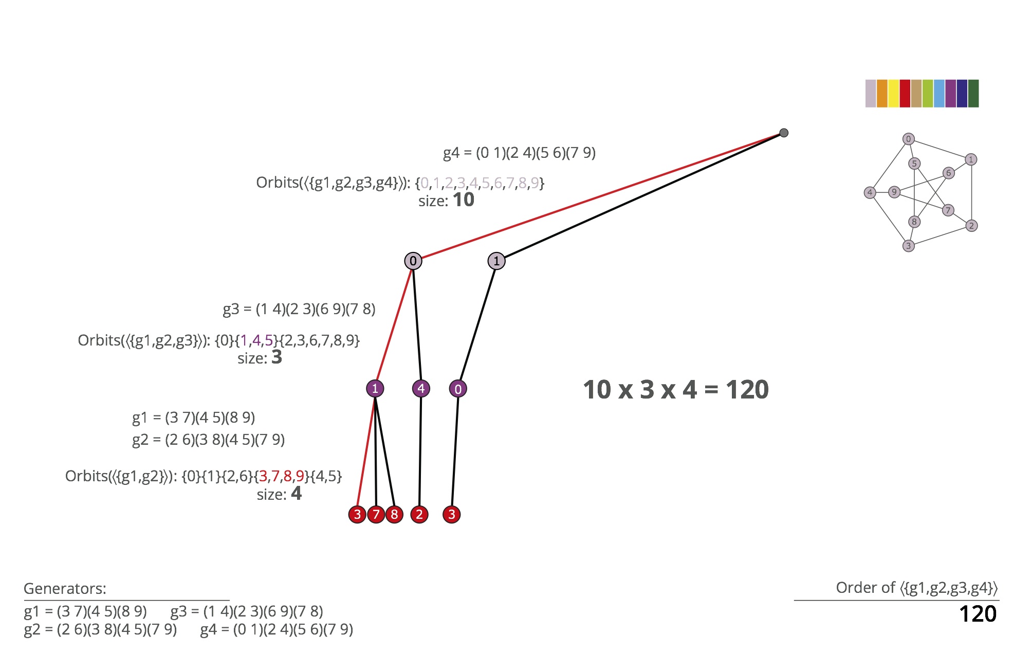
Group order. Due to the way generators are found, the group size is computed by invoking the orbit-stabilizer and Lagrange theorems. Note that the generators g1 and g2 fix 0 and 1, g3 fixes 0 and g4 maps 0 to 1.
-
-
-
Traces' search tree. The target cell has size 10 at the topmost level. At level 2, it has size 6, size 2 at level 3, where the obtained partitions are discrete. Traces executes a variant of a breadth-first traversal of the tree, pruning it as soon as automorphisms are found.
-

First individualization and refinement. The first vertex in the target cell {0,...,9} is individualized; the corresponding partition [ 0 | 1:9 ] is refined to the equitable partition [ 0 | 2 3 6:9 | 1 4 5 ]. The breadth-first search is temporarily suspended.
-

Experimental path. The computation of the first experimental path is started. After refinement, the individualization of vertex 2 produces the partition [ 0 | 2 | 8 9 | 6 | 3 7 | 4 5 | 1 ].
-
Discrete partition.
The first experimental path ends with [ 0 | 2 | 8 | 9 | 6 | 3 | 7 | 5 | 4 | 1 ], a discrete partition. -
Breadth-first resumed. The discrete partition obtained from the experimental path is stored into the node from where the path started. The breadth first search is resumed.
-
Individualization and refinement. The vertex 1 in the target cell {0,...,9} is individualized; the corresponding partition [ 1 | 0 2:9 ] is refined to the equitable partition [ 1 | 3:5 7:9 | 0 2 6 ]. The breadth-first search is temporarily suspended.
-
Experimental path. The experimental path from the current node is computed. It finally produces the discrete partition [ 1 | 8 | 7 | 4 | 9 | 5 | 3 | 2 | 0 | 6 ], which is stored into the current node itself.
-
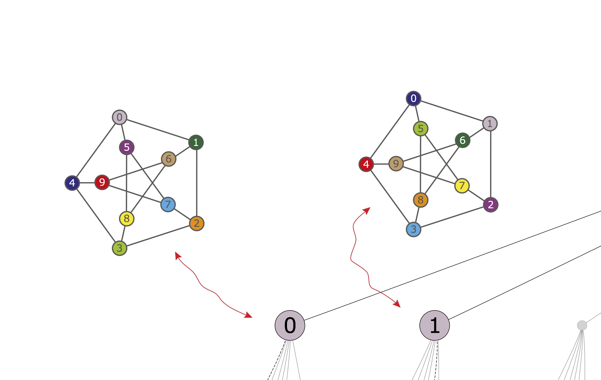
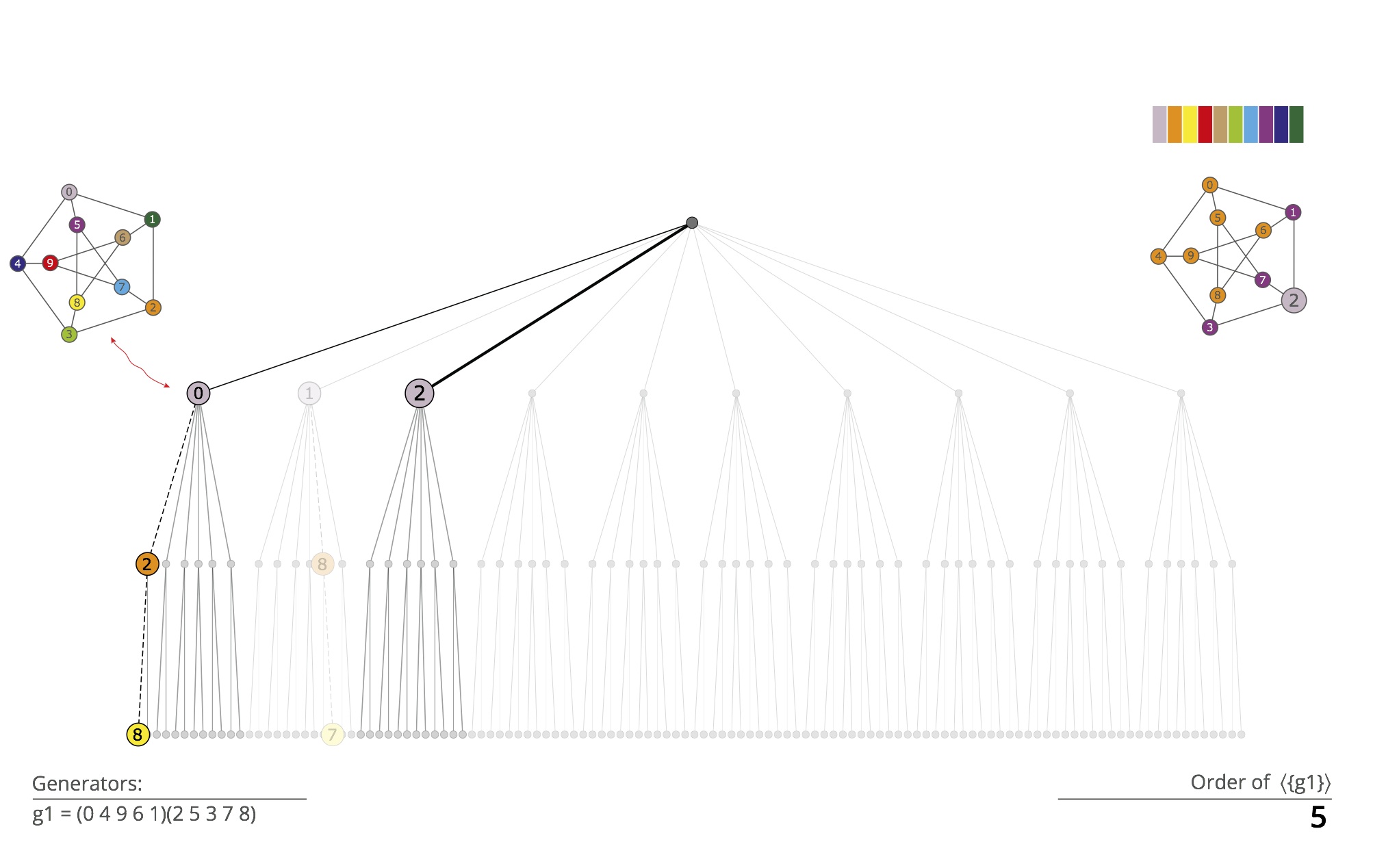
Automorphism. The discrete partitions obtained from the experimental paths are compared. An automorphism is found, g1 = (0 4 9 6 1)(2 5 3 7 8). The automorphism allows for pruning the tree in a way that at the first level, only the individualization of vertex 2 remains.
-
Individualization and refinement. The vertex 2 in the target cell {0,...,9} is individualized; the corresponding partition [ 2 | 0 1 3:9 ] is refined to the equitable partition [ 1 | 0 4:6 8 9 | 1 3 7 ]. The breadth-first search is temporarily suspended.
-
Experimental path. The experimental path from the current node is computed. It finally produces the discrete partition [ 2 | 0 | 8 | 9 | 6 | 5 | 4 | 3 | 7 | 1 ], which is stored into the current node itself.
-
Automorphism. The discrete partitions obtained from the experimental paths are compared. An automorphism is found, g2 = (0 2)(3 5)(4 7). The group ‹{g1,g2}› has order 120 and one orbit.
-
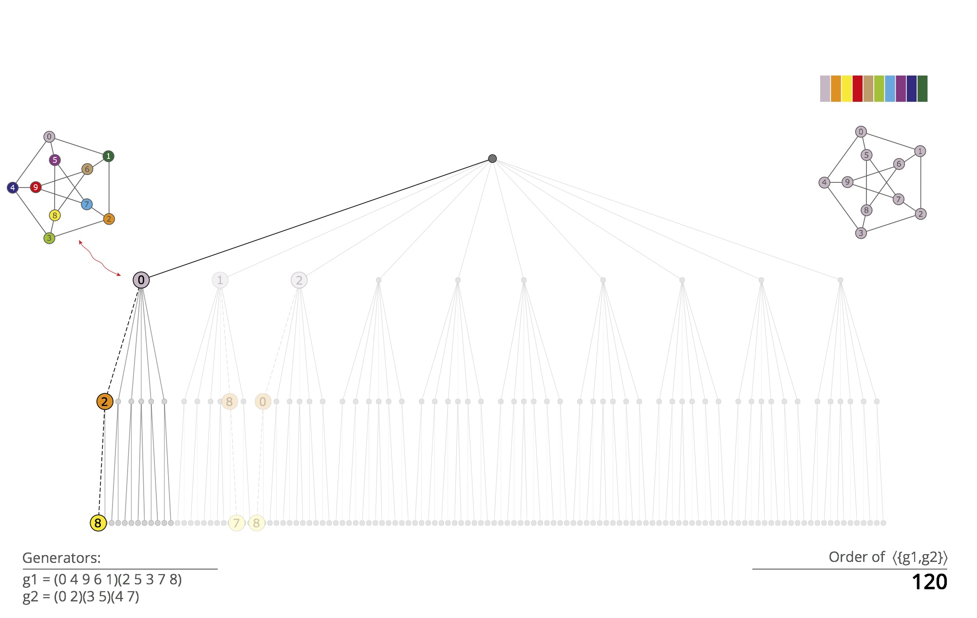
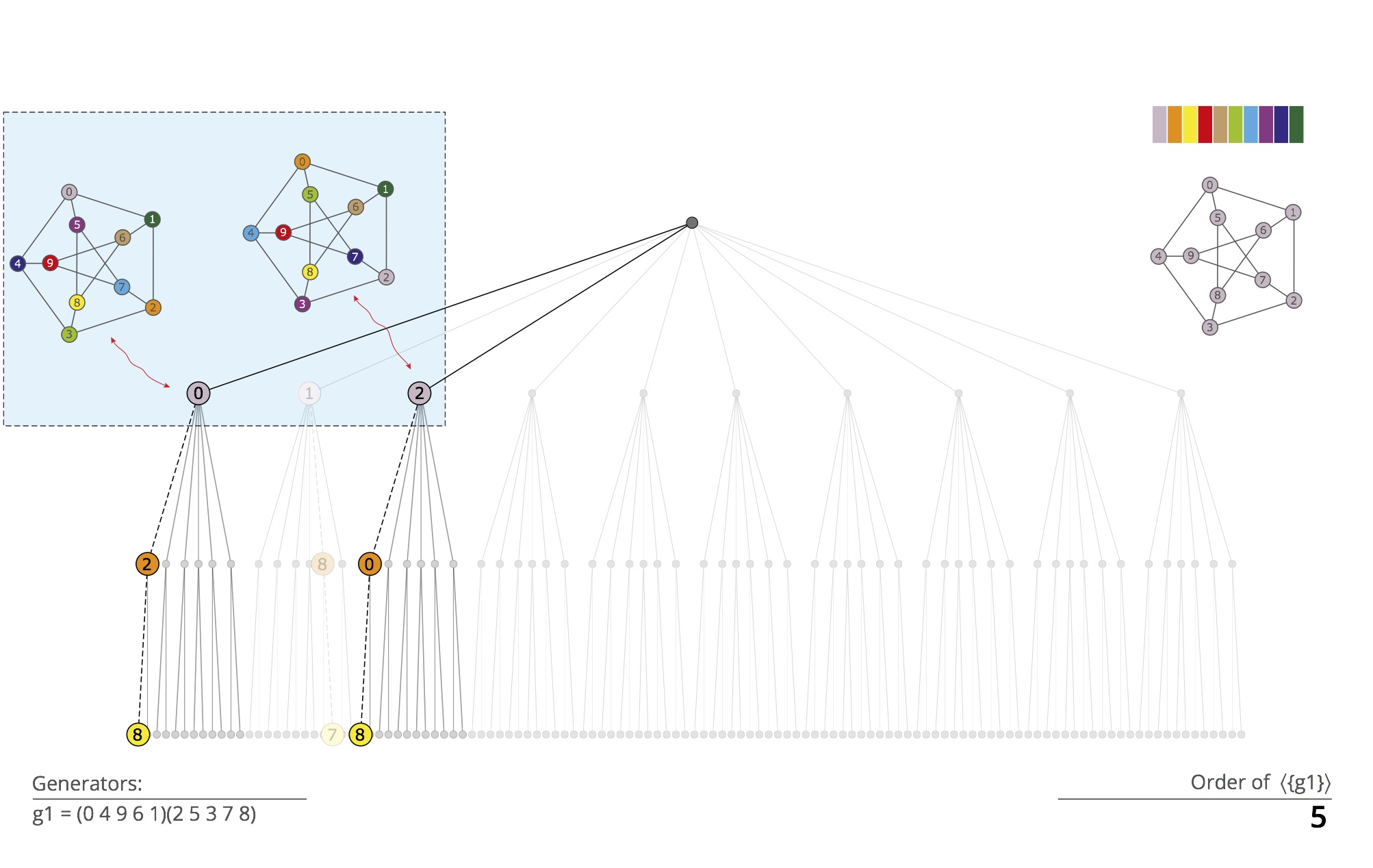
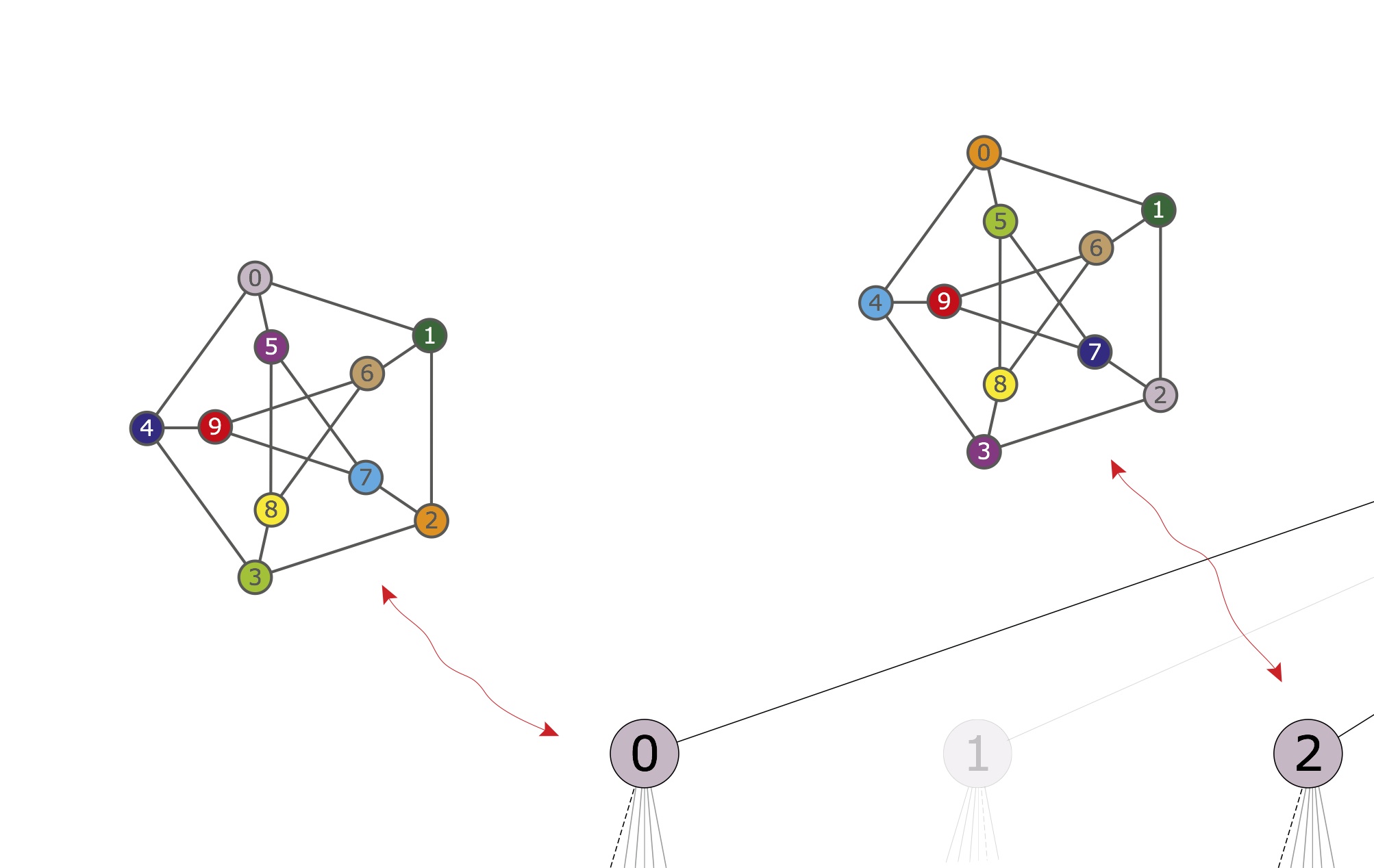
End of first level. The first level has been completed. All the nodes have been pruned except the first one. Using the Schreier-Sims method we detect that the vertices 2,3,6,7,8,9 are in the same orbit of the stabilizer of 0 in the group generated by g1 and g2.
-
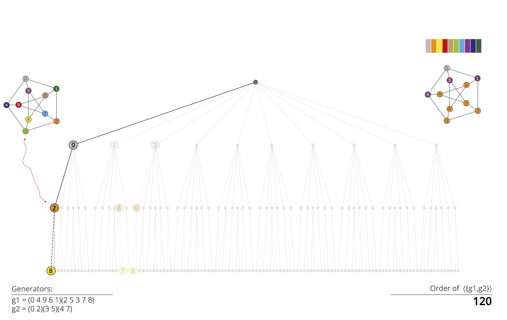
Breadth-first resumed from the second level. The target cell is here {2,3,6,7,8,9}. All these vertices are equivalent. Therefore, only vertex 2 is individualized. The partition is refined and the experimental path is computed (only if it was not computed previously).
-
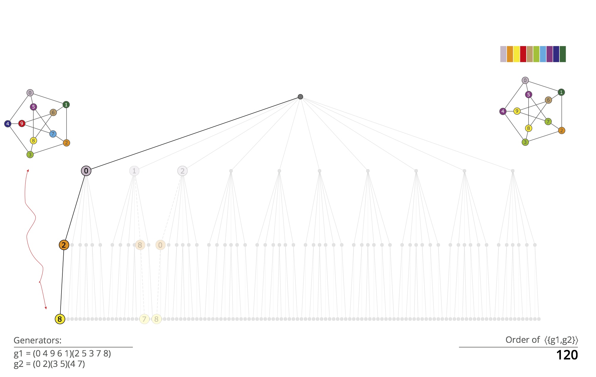
Group order. The computation proceeds to the third level, where it immediately stops after individualization of vertex 8 and refinement. The path <0,2,8> identifies the canonical labeling of the input graph. The group size is obtained by multiplying the number of vertices shown to be equivalent at level i to the i-th element of the resulting path.
-
In nauty, the search tree is generated in depth-first order. The lexicographically least leaf is kept. If the canonical labelling is sought (rather than just the automorphism group), the leaf with the greatest invariant discovered so far is also kept. Pruning operations are performed wherever possible, as high in the tree as possible.
Traces introduces an entirely different order of generating the tree, as a variant of breadth-first order.
An apparent disadvantage of breadth-first order is that pruning by automorphisms is only possible when automorphisms are known, which in general requires leaves of the tree. To remedy this problem, for every node a single path, called an ''experimental path'' is generated from that node down to a leaf of the tree.
Automorphisms are found by comparing the labelled graphs that correspond to those leaves.
We have found experimentally that generating experimental paths randomly tends to find automorphisms that generate larger subgroups, so that the group requires fewer generators altogether and more of the group is available early for pruning.
The group generated by the automorphisms found so far is maintained using the random Schreier method.